Python Object-Oriented Programming (OOP): What can we say about US housing price inflation?
Introduction
In this project, we analyze housing price inflation in the USA using object-oriented programming (OOP). Our econometric strategy is the autoregressive modeling approach. We use OOP to apply the AR process to a time series data. We consider a housing proce index:
$y_{t}$: S&P/Case-Shiller U.S. National Home Price Index
You can acess this data from https://fred.stlouisfed.org/series/CSUSHPISA. For more information regarding the index, please visit Standard & Poor's (https://www.spglobal.com/spdji/en/documents/methodologies/methodology-sp-corelogic-cs-home-price-indices.pdf). There is more information about home price sales pairs in the Methodology section. Copyright, 2016, Standard & Poor's Financial Services LLC. Reprinted with permission.
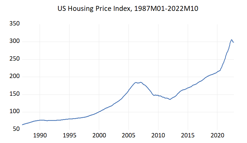
From this figure, also from unit root tests, we understand this variable is nonstationary in level. Thus, we use first difference of LOG = percentage change:
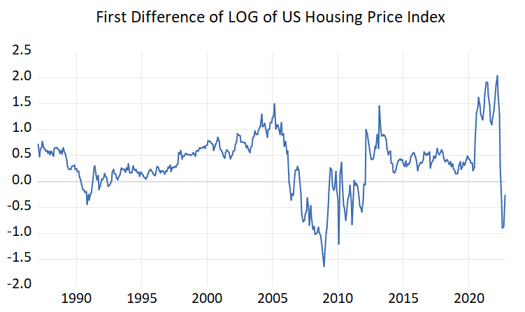
Let's make it the subject of another series of articles that this graphic tells us about the US economy. Now our priority is the processing of AR models with OOP. Let's download the necessary packages:
import numpy as np
import numpy.random as rnd
import matplotlib.pyplot as plt
from numpy import hstack, nan, tile, vstack, zeros

try:
    import seaborn
except ImportError:
    pass
Defining an AR Class
Let's create an AR class and define the methods and basic building blocks within this class.
class AR(object):
    def __init__(self, data=None, ar_order=1):
        self._data = data
        self._ar_order = ar_order
        self._sigma2 = 1
        self._T = None
        self._X = None
        self._y = None
        self._roots = None
        self._abs_roots = None
        self._fit_values = None
        self._parameters = None
        self._errors = None
        if data is not None:
            self._generate_regressor_array()

    @property
    def data(self):
        return self._data
    @property
    def ar_order(self):
        return self._ar_order
    @property
    def parameters(self):
        return self._parameters
    @property
    def sigma2(self):
        return self._sigma2
    @property
    def roots(self):
        return self._roots
    @property
    def abs_roots(self):
        return self._abs_roots
    @property
    def fit_values(self):
        if self._fit_values is None:
            self.estimate()
        return self._fit_values

    @data.setter
    def data(self, value):
        self._data = value
        self._generate_regressor_array()
        if self._parameters is not None:
            self._update_values()

    @parameters.setter
    def parameters(self, value):
        if value.ndim not in (1, 2):
            raise ValueError("parameters must be a vector")
        value = value.ravel()[:, None]
        if value.shape[0] != (self._ar_order + 1):
            raise ValueError(f"parameters must have {self._ar_order + 1} elements.")
        self._parameters = value
        self._update_roots()

    @sigma2.setter
    def sigma2(self, value):
        if value <= 0.0:
            raise ValueError("sigma2 must be positive")
        self._sigma2 = value

    def _generate_regressor_array(self):
        p = self._ar_order
        T = self._T = len(self._data)
        x = np.ones((T - p, p + 1))
        y = self._data[:, None]
        for i in range(p):
            x[:, [i + 1]] = y[p - i - 1:T - i - 1, :]
        self._y = self.data[p:, None]
        self._X = x

    def _update_roots(self):
        if self._ar_order > 0:
            coeffs = self._parameters[1:].ravel()
            char_equation = np.concatenate(([1], -1.0 * coeffs))
            self._roots = np.roots(char_equation)
            self._abs_roots = np.absolute(self._roots)
        else:
            self._roots = None
            self._abs_roots = None

    def _update_values(self):
        fv = self._X.dot(self._parameters)
        e = self._y - fv
        self._sigma2 = np.dot(e.T, e) / len(e)
        self._errors = vstack((tile(nan, (self._ar_order, 1)), e))
        self._fit_values = vstack((tile(nan, (self._ar_order, 1)), fv))

    def estimate(self, insample=None):
        x = self._X
        y = self._y
    #   y = y[:, None]
        p = self._ar_order
        if insample is not None:
            x = x[:(insample - p),:]
            y = y[:(insample - p)]
        xpxi = np.linalg.pinv(x)
        self.parameters = xpxi.dot(y)

    def forecast(self, h=1, insample=None):
        tau = self._X[:, 1:].shape[0]
        fcasts = hstack((self._X[:, :0:-1], zeros((tau, h))))
        p = self._ar_order
        params = self._parameters
        for i in range(h):
            fcasts[:, p + i] = params[0]
            for j in range(p):
                fcasts[:, p + i] += params[j + 1] * fcasts[:, p + i - (j + 1)]
        fcasts = vstack((tile(nan, (p, p + h)), fcasts))
        if insample is not None:
            fcasts[:insample, :] = nan
        return fcasts[:, p:]

    def forecast_plot(self, h=1, show=True, show_errors=False):
        fcasts = self.forecast(h=h)
        T = self._T
        p = self._ar_order
        aligned = zeros((T + h, 2))
        aligned[:T, 0] = self._data
        aligned[-T:, 1] = fcasts[:, -1]
        aligned = aligned[p:T, :]
        fig = plt.figure()
        ax = fig.add_subplot(1, 1, 1)
        if show_errors:
            ax.plot(aligned[:, 0] - aligned[:, 1])
        else:
            ax.plot(aligned)
        if show:
            plt.show(fig)
        return fig

    def hedgehog_plot(self, h=1, show=True, skip=0):
        fcasts = self.forecast(h=h)
        fig = plt.figure()
        ax = fig.add_subplot(1, 1, 1)
        ax.plot(self._data)
        data = self._data
        for i in range(0, self._T, skip + 1):
            x = i + np.arange(h + 1)
            y = hstack((data[[i]], fcasts[i]))
            ax.plot(x, y, 'r')
        ax.autoscale(tight='x')
        fig.tight_layout()
        if show:
            plt.show(fig)
        return fig

    def simulate(self, T=500, burnin=500):
        tau = T + burnin + self._ar_order
        e = rnd.standard_normal((tau,))
        y = zeros((tau,))
        p = self._ar_order
        for t in range(p, tau):
            y[t] = self._parameters[0]
            for i in range(p):
                y[t] += self._parameters[i + 1] * y[t - i - 1]
            y[t] += e[t]
        return y[-T:]
Load the data
import pandas as pd

housinginf_excel = pd.read_excel("housinginf.xls", skiprows=10,
                           index_col="observation_date")

# print(gs10_excel)
data = housinginf_excel.housinginf.to_numpy()
We estimate the following model with the estimation and forecasting methods we defined in the AR class: $$y_{t}=\alpha_{0}+\alpha_{1}y_{t-1}+\alpha_{2}y_{t-2}+\alpha_{3}y_{t-3}+\varepsilon_{t}$$
T = 429
ar_order = 3
in_sample = 10
h=5
# Initialize the object
# ar = AR(activity, ar_order)
ar=AR(data,ar_order)
ar.estimate()
forecasts = ar.forecast(h,in_sample)
Let's plot the forecasting error data with the real data:
p = ar_order
aligned = zeros((T + h, 2))
aligned[:T, 0] = data
aligned[-T:, 1] = forecasts[:, -1]
aligned = aligned[p:T, :]

plt.plot(np.arange(1, T-ar_order+1), aligned)
plt.show()

In this figure, the blue series represents the actual data, while the orange series represents the forecast error data. Note: The information in the link below was used in the creation of the OOP for the AR modeling approach: https://www.kevinsheppard.com/teaching/python/notes/#notes