Modeling the VIX index
In this post, we want to determine which model structure is convenient for analyzing the VIX index? Let consider out data comprise SP500, Dow Jones indexes and Treasury bill rate İN US.Our time series data are monthly and from 2000M1-2021M08.
First we set the work directory:
```{r setup, include=FALSE}
if(!is.null(dev.list())) dev.off() cat(“\014”) rm(list=ls(all=TRUE))
Current directory
setwd(“C:/Users/Admin/Desktop/web page halil/posts/1”)
```{r}
# You should install this packages:

install.packages("readxl")
install.packages("xlsx")
install.packages("tidyverse")
install.packages("xts")
install.packages("zoo")
install.packages("tsutils")
install.packages("urca")
install.packages("aTSA")
install.packages("erer")
install.packages("calibrate")
install.packages("pracma")
install.packages("caret")
library(readxl)
library(xlsx)
library(tidyverse)
library(xts)
library(zoo)
library(tsutils)
library(urca)
library(aTSA)
library(erer)
library(calibrate)
library(pracma)
library(caret)
# call data from xlsx file

data <- read_excel(file <- "data.xlsx")
From data.xlsx file the data description is as follows: sp:SP500 Index (index level points) dj:Dow Jones Index (index level points) VİX: VIX index (index level points) tb: Treasury Bill Rate (in %)
Outlier detection
In this trial, We use the Hampel filter to detect outliers in these time series. It uses a sliding window of configurable width to go over the data. In the method, the sliding window lengths are fixed. In addition, the median absolute deviation (MAD) is used. You can find detailed information from Liu, H., Shah, S., & Jiang, W. (2004). On-line outlier detection and data cleaning. Computers & chemical engineering, 28(9), 1635-1647.
X01 <- cbind(data$sp)

End01 <- nrow(X01)

Len <- 5
X11 <- c(numeric(Len-1), X01)
win1 <- matrix(list(), 1, End01)
m1 <- t(numeric(End01))
sigma1 <- t(numeric(End01))
mad1 <- t(numeric(End01))
kappa <- 1.4826
nsigma <- 2
mutlax1 <- matrix(list(), 1, End01)
deg1 <- t(numeric(End01))
comp1 <- t(numeric(End01))

for(e in 1:End01) {
  win1[[1,e]] <- X11[e:(e+Len-1)]
  m1[e] <- median(win1[[1,e]])
  mad1[e] <- median(abs(win1[[1,e]]-median(m1[e])))
  sigma1[e] <- kappa*mad1[e]
  mutlax1[[1,e]] <- abs(win1[[1,e]]-m1[e])
  deg1[e] <- nsigma*sigma1[e]
  comp1[e] <- mutlax1[[1,e]][(Len-1)/2+1]
}

l <- (Len-1)/2
s1 <- numeric(End01-l)
for (ii in 1+l:End01) {
    ifelse(comp1[ii] > deg1[ii],s1[ii] <- 1,s1[ii] <- 0)
}
s1 <- s1[(1+l):length(s1)]
outlier1 <- !(!s1)
outlierX01 <- X01[outlier1]
outlierX01

These values are outliers for SP500 index series.
X02 <- cbind(data$dj)
X02 <- cbind(X02[!is.na(X02)])
End02 <- nrow(X02)

X12 <- c(numeric(Len-1), X02)
win2 <- matrix(list(), 1, End02)
m2 <- t(numeric(End02))
sigma2 <- t(numeric(End02))
mad2 <- t(numeric(End02))
mutlax2 <- matrix(list(), 1, End02)
deg2 <- t(numeric(End02))
comp2 <- t(numeric(End02))

for(e in 1:End02) {
  win2[[1,e]] <- X12[e:(e+Len-1)]
  m2[e] <- median(win2[[1,e]])
  mad2[e] <- median(abs(win2[[1,e]]-median(m2[e])))
  sigma2[e] <- kappa*mad2[e]
  mutlax2[[1,e]] <- abs(win2[[1,e]]-m2[e])
  deg2[e] <- nsigma*sigma2[e]
  comp2[e] <- mutlax2[[1,e]][(Len-1)/2+1]
}

s2 <- numeric(End02-l)
for (ii in 1+l:End02) {
    ifelse(comp2[ii] > deg2[ii],s2[ii] <- 1,s2[ii] <- 0)
}
s2 <- s2[(1+l):length(s2)]
outlier2 <- !(!s2)
outlierX02 <- X02[outlier2]
outlierX02

These values are outliers for Dow Jones index series.
X03 <- cbind(data$vix)
X03 <- X03[121:nrow(X03)]
X03 <- cbind(na.locf(X03))

End03 <- nrow(X03)

X13 <- c(numeric(Len-1), X03)
win3 <- matrix(list(), 1, End03)
m3 <- t(numeric(End03))
sigma3 <- t(numeric(End03))
mad3 <- t(numeric(End03))
mutlax3 <- matrix(list(), 1, End03)
deg3 <- t(numeric(End03))
comp3 <- t(numeric(End03))

for(e in 1:End03) {
  win3[[1,e]] <- X13[e:(e+Len-1)]
  m3[e] <- median(win3[[1,e]])
  mad3[e] <- median(abs(win3[[1,e]]-median(m3[e])))
  sigma3[e] <- kappa*mad3[e]
  mutlax3[[1,e]] <- abs(win3[[1,e]]-m3[e])
  deg3[e] <- nsigma*sigma3[e]
  comp3[e] <- mutlax3[[1,e]][(Len-1)/2+1]
}

s3 <- numeric(End03-l)
for (ii in 1+l:End03) {
    ifelse(comp3[ii] > deg3[ii],s3[ii] <- 1,s3[ii] <- 0)
}
s3 <- s3[(1+l):length(s3)]
outlier3 <- !(!s3)
outlierX03 <- X03[outlier3]
outlierX03

These values are outliers for VIX index series.
X04 <- cbind(data$tb)
X04 <- X04[119:nrow(X04)]
X04 <- cbind(na.locf(X04))
End04 <- nrow(X04)

X14 <- c(numeric(Len-1), X04)
win4 <- matrix(list(), 1, End04)
m4 <- t(numeric(End04))
sigma4 <- t(numeric(End04))
mad4 <- t(numeric(End04))
mutlax4 <- matrix(list(), 1, End04)
deg4 <- t(numeric(End04))
comp4 <- t(numeric(End04))

for(e in 1:End04) {
  win4[[1,e]] <- X14[e:(e+Len-1)]
  m4[e] <- median(win4[[1,e]])
  mad4[e] <- median(abs(win4[[1,e]]-median(m4[e])))
  sigma4[e] <- kappa*mad4[e]
  mutlax4[[1,e]] <- abs(win4[[1,e]]-m4[e])
  deg4[e] <- nsigma*sigma4[e]
  comp4[e] <- mutlax4[[1,e]][(Len-1)/2+1]
}

s4 <- numeric(End04-l)
for (ii in 1+l:End04) {
    ifelse(comp4[ii] > deg4[ii],s4[ii] <- 1,s4[ii] <- 0)
}
s4 <- s4[(1+l):length(s4)]
outlier4 <- !(!s4)
outlierX4 <- X04[outlier4]
outlierX4

These values are outliers for treasury bill rate.
Modelling the VIX index
Let’s create a simple quarterly model that explains the VIX index. In doing so, our potential independent variables are sp500, dj, and tb. After providing a measure of how our alternative models are performing (in-sample), let’s select and interpret the one that best fits the vix data.
First, the stationary properties of the series must be determined. Let’s apply the ADF unit root test to the level values of the series. Then, the ADF test is performed on the first differences of series. In all tests, ADF unit root test functional patterns are constant and both constant and trend.
veri01 <- cbind(data$sp,data$dj,data$vix,data$tb)
K <- ncol(veri01)
T <- nrow(veri01)
pmax <- round((12*((T/100)^(1/4))), digits = 0)
S0 <- matrix(nrow = K, ncol = 1,0)
S1 <- matrix(nrow = K, ncol = 1,0)
sonuc_ur <- matrix(nrow = K, ncol = 2,0)

for (k in 1:K) {
    sonucADF_cons <- ur.df2(veri01[,k], type = c("drift"), lags = pmax,
      selectlags = c("BIC"), digit = 2)
    sonucADF_trend <- ur.df2(veri01[,k], type = c("trend"), lags = pmax,
      selectlags = c("BIC"), digit = 2)
    if (sonucADF_cons$teststat[1,1]<sonucADF_cons$cval[1,2]){
      sonuc_ur[k,1] <- 1
      } else {
      sonuc_ur[k,1] <- 0
      }
    if (sonucADF_trend$teststat[1,1]<sonucADF_trend$cval[1,2]){
      sonuc_ur[k,2] <- 1
      } else {
      sonuc_ur[k,2] <- 0
      }
}

sonuc_ur_1 <- matrix(nrow = K, ncol = 2,0)

for (k in 1:K) {
    sonucADF_cons1 <- ur.df2(diff(veri01[,k],1), type = c("drift"), lags = pmax,
      selectlags = c("BIC"), digit = 2)
    sonucADF_trend1 <- ur.df2(diff(veri01[,k],1), type = c("trend"), lags = pmax,
      selectlags = c("BIC"), digit = 2)
    if (sonucADF_cons1$teststat[1,1] < sonucADF_cons1$cval[1,2]){
      sonuc_ur_1[k,1] <- 1
      } else {
      sonuc_ur_1[k,1] <- 0
      }
    if (sonucADF_trend1$teststat[1,1] < sonucADF_trend1$cval[1,2]){
      sonuc_ur_1[k,2] <- 1
      } else {
      sonuc_ur_1[k,2] <- 0
      }
}

sonuc_ur
sonuc_ur_1
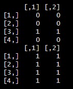
This table shows that the series are stationary at their difference values.
Transformation of series:
x3 <- cbind(veri01[,3])
x3 <- x3[2:nrow(veri01)]
z1 <- 100*(log(veri01[,1])-log(lag(veri01[,1],1)))
z2 <- 100*(log(veri01[,2])-log(lag(veri01[,2],1)))
z4 <- 100*(sign(veri01[,4])*log(1+abs(veri01[,4]))-sign(lag(veri01[,4],1))*log(1+abs(lag(veri01[,4],1))))

Z <- cbind(ones(T-1,1),z1[-1],z2[-1],z4[-1])
Since there are 3 independent variables in the model, there are 7 different model alternatives: \(\begin{split} vix &= f(sp) , \\ vix &= f(dj) , \\ vix &= f(tb) , \\ vix &= f(sp,dj) , \\ vix &= f(sp,tb) , \\ vix &= f(dj,tb) , \\ vix &= f(sp,dj,tb) , \end{split}\)
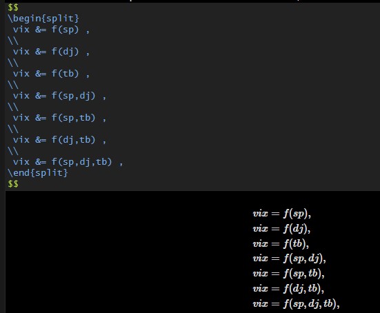
With the coding given below, we estimate all these models and compare the in-sample predictions of the models with adjusted R2:
W <- 7
ZZ <- matrix(list(), 1, W)
a <- cbind(2,3,4)
R <- matrix(list(), 1, ncol(a)+1)
res <- unlist(lapply(1:3, combn,
                     x = c(2,3,4), simplify = FALSE),
              recursive = FALSE)
res <- sapply(res, `length<-`, 3)
adjR2s <- matrix(nrow = W, ncol = 1,0)
for (w in 1:W){
  ZZ[[1,w]] <- Z[,na.omit(res[,w])]
  adjR2s[w] <- summary(lm(x3~ZZ[[1,w]]))$adj.r.squared
}


ModelNumber <- which.max(adjR2s)
bestModel <- lm(x3~ZZ[[1,ModelNumber]])

summary(bestModel)
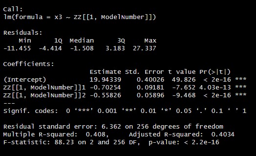
As a result, the model with sp and dj variables is the most successful. With the individual parameter estimations of this model, the significance of the model is proved statistically. Economically, the growth rate of the sp and dj series decreases the growth rate of the vix index. The VIX index is an indicator of volatility in the markets. In this case, since the sp and dj index shows the development of the markets, the findings are economically consistent.
Note: The Cboe Volatility Index (VIX) signals the level of fear or stress in the stock market